Know what the series is doing
before you pick a model.
Trend, seasonality, and whether anything actually beats naive — answered in seconds, without writing the boilerplate first. You can build all of this yourself; that's not the point. This is the triage pass before you commit to an approach.
Decompose · Compare methods · Beat naive
From spreadsheet to forecast in under 30 seconds
Paste a column of history, pick a method, read the range. No setup, no scripting.
The first look costs more than it should
The modelling isn't hard. It's the scaffolding you write before you know whether the series is even worth modelling that eats the afternoon.
Boilerplate before signal
Load, resample, split, fit, plot — a lot of setup just to answer "is there a trend here at all?"
No cheap baseline
Beating naive is the first question anyone should ask, and the last thing anyone actually wires up.
Seasonality stays a guess
You suspect a 12-period cycle, but confirming it means a decomposition detour before the real work starts.
Diagnose the series, then score every method against it
Paste a series and get an immediate read: profile, decomposition, and the whole method library fit and ranked side by side — with in-sample fit, out-of-sample backtests, and the parameters each method landed on. Inspectable, not a black box.
- Instant series profile — N, min, mean, max, σ and the shape of the data before you model anything.
- STL decomposition — trend, seasonal and residual components — with an independent seasonality training window when the pattern is longer than your lookback.
- Method sweep, ranked — Holt-Winters (additive / multiplicative / auto), linear & log trend, growth rate, moving average and more, scored in one table.
- Rolling-origin backtests — R², MAPE, RMSE, MAE, bias and interval coverage per method — held-out evaluation without writing the split loop.
 Forecast Lab · Air Passengers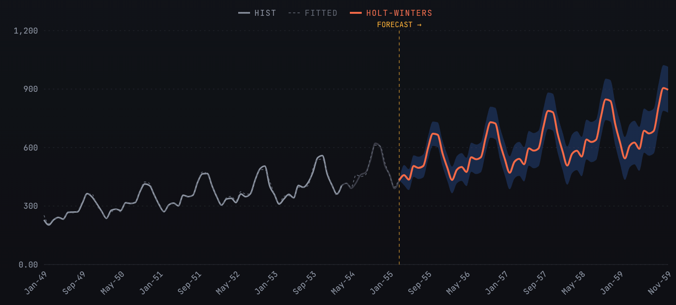
When the answer is a range, not a number
If the triage pass says the uncertainty matters more than the point estimate, define variables, distributions and formulas in a live graph and run up to 10,000 paths — no simulator to write.
- Distribution-driven variables — normal, lognormal and more, with per-period resampling and bounds.
- Formula graph — dependency-resolved cells combining forecasts, assumptions and derived metrics.
- Full output distributions — mean, std, CV, KDE and P10 / P50 / P90 rather than a point estimate.
- Export the results — pull the numbers back out when the quick pass turns into real work.
Monte Carlo Lab · 5,000 sims · h=36From raw series to a decision about the approach
Three steps. No setup, no scripting. Just forecasts.
Paste or upload the series
Instant profiling — N, min, mean, max, σ — before you model anything.
Read the diagnostics
Decompose for trend and seasonality, then compare every method's out-of-sample error against naive.
Decide the approach
Take the winning direction back to the notebook, or export the numbers and keep going.
The honest answers
“Doesn't statsmodels already do this?”
Yes — and this doesn't replace it. It replaces the first hour of scaffolding you write before you know which direction is worth pursuing.
“Does anything here actually beat naive?”
That's the point of the fit table. Every method is scored on held-out data side by side, so a flat baseline winning is a real, visible result.
“Can I see how the fit was evaluated?”
Out-of-sample metrics, fitted parameters, residual decomposition and interval coverage are all exposed per method.
Keep the triage passes you already ran
Save each quick look into a workspace so you're not re-pasting the same series next month. And when someone asks to see it, share a link — they get the interactive forecast with the accuracy metrics attached, instead of a screenshot from your notebook.
Triage the series first.
Then pick your model.
Decomposition, a full method sweep and out-of-sample metrics in the browser — before you write a line of code.
20 minutes · Your data questions answered live